deweather is an R package developed for the purpose of “removing” the influence of meteorology from air quality time series data. It is part of the openair suite of packages designed to support the analysis of air quality data and related data.
The deweather package uses a boosted regression tree approach for modelling air quality data. These and similar techniques provide powerful tools for building statistical models of air quality data. They are able to take account of the many complex interactions between variables as well as non-linear relationships between the variables.
The modelling can be computationally intensive and therefore deweather makes use of the parallel processing, which should work on Windows, Linux and Mac OSX.
Installation
Installation of deweather from GitHub should be easy using the pak package.
# install.packages("pak")
pak::pak("davidcarslaw/deweather")
Description
Meteorology plays a central role in affecting the concentrations of pollutants in the atmosphere. When considering trends in air pollutants it can be very difficult to know whether a change in concentration is due to emissions or meteorology.
The deweather package uses a powerful statistical technique based on boosted regression trees using the gbm package (Ridgeway, 2017). Statistical models are developed to explain concentrations using meteorological and other variables. These models can be tested on randomly withheld data with the aim of developing the most appropriate model.
Example data set
The deweather package comes with a comprehensive data set of air quality and meteorological data. The air quality data is from Marylebone Road in central London (obtained from the openair package) and the meteorological data from Heathrow Airport (obtained from the worldmet package).
The road_data data frame contains various pollutants such a NOx, NO2, ethane and isoprene as well as meteorological data including wind speed, wind direction, relative humidity, ambient temperature and cloud cover. Code to obtain this data directly can be found here.
library(deweather)
head(road_data)
#> # A tibble: 6 × 11
#>   date                  nox   no2 ethane isoprene benzene    ws    wd air_temp
#>   <dttm>              <dbl> <dbl>  <dbl>    <dbl>   <dbl> <dbl> <dbl>    <dbl>
#> 1 1998-01-01 00:00:00   546    74     NA       NA      NA   1     280     3.6
#> 2 1998-01-01 01:00:00    NA    NA     NA       NA      NA   1     230     3.5
#> 3 1998-01-01 02:00:00    NA    NA     NA       NA      NA   1.5   180     4.25
#> 4 1998-01-01 03:00:00   944    99     NA       NA      NA  NA      NA    NA
#> 5 1998-01-01 04:00:00   894   149     NA       NA      NA   1.5   180     3.8
#> 6 1998-01-01 05:00:00   506    80     NA       NA      NA   1     190     3.5
#> # ℹ 2 more variables: RH <dbl>, cl <dbl>
Construct and test model(s)
The testMod() function is used to build and test various models to help derive the most appropriate.
In this example, we will restrict the data to model to 4 years. Note that variables such as "hour" and "weekday" are used as variables that can be used to explain some of the variation. "hour" for example very usefully acts as a proxy for the diurnal variation in emissions.
library(openair)
# select only part of the data set
dat_part <- selectByDate(road_data, year = 2001:2004)

# test a model with commonly used covariates
testMod(
  dat_part,
  vars = c("trend", "ws", "wd", "hour", "weekday", "air_temp", "week"),
  pollutant = "no2"
)
#> ℹ Optimum number of trees is 2483
#> ℹ RMSE from cross-validation is 20.97
#> ℹ Percent increase in RMSE using test data is 33.3%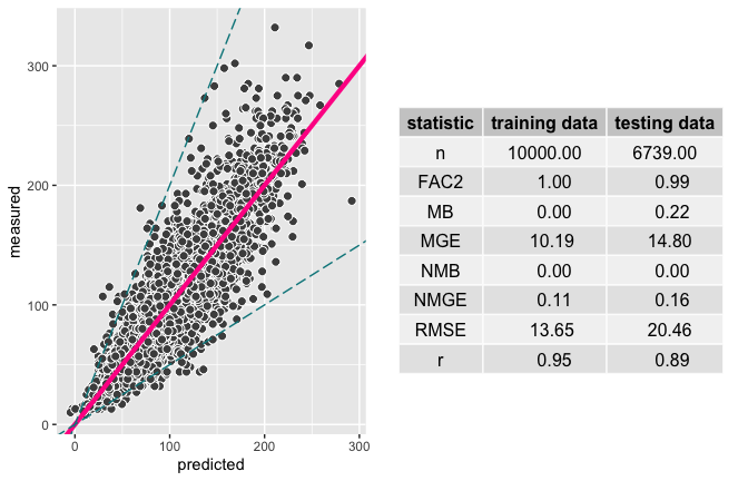
A statistical summary of a deweather model test.
The output shows by default the performance of the model when applied to a withheld random 20% (by default) of the data, i.e., the model is evaluated against data not used to build the model. Common model evaluation metrics are also given.
Build a model
Assuming that a good model can be developed, it can now be explored in more detailusing the optinum number of trees from testMod..
mod_no2 <- buildMod(
  dat_part,
  vars = c("trend", "ws", "wd", "hour", "weekday", "air_temp", "week"),
  pollutant = "no2",
  n.trees = 2483,
  n.core = 6
)
This function returns a deweather object that can be interrogated as shown below.
Examine the partial dependencies
Plot all partial dependencies
One of the benefits of the boosted regression tree approach is that the partial dependencies can be explored. In simple terms, the partial dependencies show the relationship between the pollutant of interest and the covariates used in the model while holding the value of other covariates at their mean level.
plotPD(mod_no2, nrow = 4)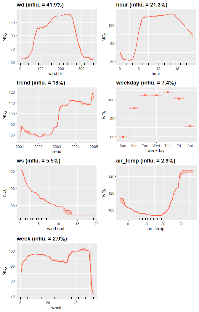
The 7 partial dependencies of the deweather model.
Plot two-way interactions
It can be very useful to plot important two-way interactions. In this example the interaction between "ws" and "air_temp" is considered. The plot shows that NO2 tends to be high when the wind speed is low and the temperature is low, i.e., stable atmospheric conditions. Also NO2 tends to be high when the temperature is high, which is most likely due to more O3 available to convert NO to NO2. In fact, background O3 would probably be a useful covariate to add to the model.
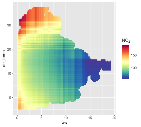
A two-way interaction plot showing the interaction between wind speed and air temperature
Apply meteorological averaging
An indication of the meteorologically-averaged trend is given by the plotAllPD() function above. A better indication is given by using the model to predict many times with random sampling of meteorological conditions. This sampling is carried out by the metSim() function. Note that in this case there is no need to supply the "trend" component because it is calculated using metSim().
demet <- metSim(mod_no2,
  newdata = dat_part,
  metVars = c("ws", "wd", "hour", "weekday", "air_temp", "week")
)
Now it is possible to plot the resulting trend.
library(ggplot2)
ggplot(demet, aes(date, no2)) +
  geom_line() +
  labs(y = quickText("Deweathered no2 (ug/m3)"))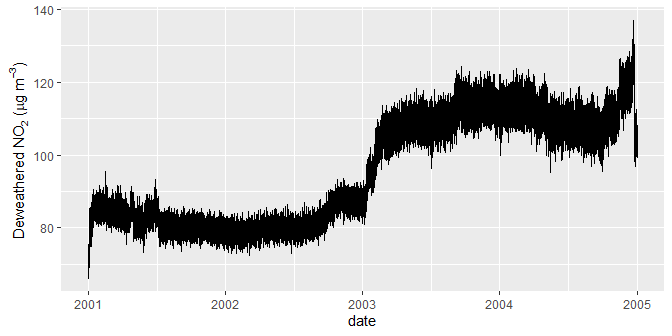
A deweathered nitrogen dioxide trend.
The plot is rather noisy due to relatively few samples of meteorology being considered (200 by default, set with B = 200). The noise could be reduced by increasing the simulations, but this would add to run time. Alternatively, it can be useful to simply average the results. For example:
library(ggplot2)
ggplot(timeAverage(demet, "day"), aes(date, no2)) +
  geom_line(col = "dodgerblue", size = 1) +
  labs(y = quickText("Deweathered NO2 (ug/m3)"))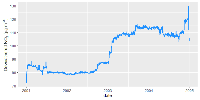
A time-averaged deweathered nitrogen dioxide trend.
References
Grange, S. K. and Carslaw, D. C. (2019) Using meteorological normalisation to detect interventions in air quality time series, Science of The Total Environment. 653, pp. 578–588. doi: 10.1016/j.scitotenv.2018.10.344.
Carslaw, D.C., Williams, M.L. and B. Barratt (2012) A short-term intervention study — impact of airport closure on near-field air quality due to the eruption of Eyjafjallajökull, Atmospheric Environment, Vol. 54, 328–336.
Carslaw, D.C. and P.J. Taylor (2009). Analysis of air pollution data at a mixed source location using boosted regression trees, Atmospheric Environment. Vol. 43, pp. 3563–3570.
Greenwell B, Boehmke B, Cunningham J, Developers G (2022). gbm: Generalized Boosted Regression Models. R package version 2.1.8.1, https://CRAN.R-project.org/package=gbm.