openair is an R package developed for the purpose of analysing air quality data — or more generally atmospheric composition data. The package is extensively used in academia, the public and private sectors. The project was initially funded by the UK Natural Environment Research Council (NERC), with additional funds from Defra.
The most up to date information on openair can be found in the package itself and at the book website (https://bookdown.org/david_carslaw/openair/).
Installation
Installation can be done in the normal way:
install.packages("openair")The development version can be installed from GitHub. Installation of openair from GitHub is easy using the pak package. Note, because openair contains C++ code a compiler is also needed. For Windows - for example, Rtools is needed.
# install.packages("pak")
pak::pak("davidcarslaw/openair")
Description
openair has developed over several years to help analyse air quality data.
This package continues to develop and input from other developers would be welcome. A summary of some of the features are:
-
Access to data from several hundred UK air pollution monitoring sites through the
importAURNand family functions. -
Utility functions such as
timeAverageandselectByDateto make it easier to manipulate atmospheric composition data. - Flexible wind and pollution roses through
windRoseandpollutionRose. - Flexible plot conditioning to easily plot data by hour or the day, day of the week, season etc. through the
openairtypeoption available in most functions. - More sophisticated bivariate polar plots and conditional probability functions to help characterise different sources of pollution. A paper on the latter is available here.
- Access to NOAA Hysplit pre-calculated annual 96-hour back trajectories and many plotting and analysis functions e.g. trajectory frequencies, Potential Source Contribution Function and trajectory clustering.
- Many functions for air quality model evaluation using the flexible methods described above e.g. the
typeoption to easily evaluate models by season, hour of the day etc. These include key model statistics, Taylor Diagram, Conditional Quantile plots.
Brief examples
Import data from the UK Automatic Urban and Rural Network
It is easy to import hourly data from 100s of sites and to import several sites at one time and several years of data.
library(openair)
kc1 <- importAURN(site = "kc1", year = 2020)
kc1
#> # A tibble: 8,784 × 15
#>    source site     code  date                   co   nox   no2    no    o3   so2
#>    <chr>  <chr>    <chr> <dttm>              <dbl> <dbl> <dbl> <dbl> <dbl> <dbl>
#>  1 aurn   London … KC1   2020-01-01 00:00:00 0.214  64.8  46.2 12.1   1.13    NA
#>  2 aurn   London … KC1   2020-01-01 01:00:00 0.237  74.1  45.0 19.0   1.20    NA
#>  3 aurn   London … KC1   2020-01-01 02:00:00 0.204  60.5  41.4 12.4   1.50    NA
#>  4 aurn   London … KC1   2020-01-01 03:00:00 0.204  53.5  39.8  8.93  1.60    NA
#>  5 aurn   London … KC1   2020-01-01 04:00:00 0.169  37.7  33.6  2.63  5.79    NA
#>  6 aurn   London … KC1   2020-01-01 05:00:00 0.160  43.3  36.8  4.25  6.09    NA
#>  7 aurn   London … KC1   2020-01-01 06:00:00 0.157  48.2  39.4  5.76  2.74    NA
#>  8 aurn   London … KC1   2020-01-01 07:00:00 0.178  60.5  44.7 10.3   1.20    NA
#>  9 aurn   London … KC1   2020-01-01 08:00:00 0.233  71.8  47.9 15.6   2.25    NA
#> 10 aurn   London … KC1   2020-01-01 09:00:00 0.329 128.   46.9 53.2   2.25    NA
#> # ℹ 8,774 more rows
#> # ℹ 5 more variables: pm10 <dbl>, pm2.5 <dbl>, ws <dbl>, wd <dbl>,
#> #   air_temp <dbl>
Utility functions
Using the selectByDate function it is easy to select quite complex time-based periods. For example, to select weekday (Monday to Friday) data from June to September for 2012 and for the hours 7am to 7pm inclusive:
sub <- selectByDate(kc1,
  day = "weekday",
  year = 2020,
  month = 6:9,
  hour = 7:19
)
sub
#> # A tibble: 1,144 × 15
#>    date                source site    code      co   nox   no2    no    o3   so2
#>    <dttm>              <chr>  <chr>   <chr>  <dbl> <dbl> <dbl> <dbl> <dbl> <dbl>
#>  1 2020-06-01 07:00:00 aurn   London… KC1   0.125   23.1 16.8  4.14   56.5  2.29
#>  2 2020-06-01 08:00:00 aurn   London… KC1   0.133   25.2 17.8  4.79   61.7  2.68
#>  3 2020-06-01 09:00:00 aurn   London… KC1   0.119   15.6 12.2  2.22   75.8  2.35
#>  4 2020-06-01 10:00:00 aurn   London… KC1   0.104   13.8 11.1  1.79   87.1  1.57
#>  5 2020-06-01 11:00:00 aurn   London… KC1   0.0956  14.0 11.8  1.46   96.7  1.44
#>  6 2020-06-01 12:00:00 aurn   London… KC1   0.0985  11.3  9.97 0.893 106.   1.44
#>  7 2020-06-01 13:00:00 aurn   London… KC1   0.0927  11.0  9.64 0.893 112.   2.03
#>  8 2020-06-01 14:00:00 aurn   London… KC1   0.0927  12.5 10.8  1.14  114.   2.81
#>  9 2020-06-01 15:00:00 aurn   London… KC1   0.0811  10.7  9.48 0.822 115.   2.88
#> 10 2020-06-01 16:00:00 aurn   London… KC1   0.0898  13.9 11.9  1.29  104.   2.22
#> # ℹ 1,134 more rows
#> # ℹ 5 more variables: pm10 <dbl>, pm2.5 <dbl>, ws <dbl>, wd <dbl>,
#> #   air_temp <dbl>
Similarly it is easy to time-average data in many flexible ways. For example, 2-week means can be calculated as
sub2 <- timeAverage(kc1, avg.time = "2 week")The type option
One of the key aspects of openair is the use of the type option, which is available for almost all openair functions. The type option partitions data by different categories of variable. There are many built-in options that type can take based on splitting your data by different date values. A summary of in-built values of type are:
- “year” splits data by year
- “month” splits variables by month of the year
- “monthyear” splits data by year and month
- “season” splits variables by season. Note in this case the user can also supply a
hemisphereoption that can be either “northern” (default) or “southern” - “weekday” splits variables by day of the week
- “weekend” splits variables by Saturday, Sunday, weekday
- “daylight” splits variables by nighttime/daytime. Note the user must supply a
longitudeandlatitude - “dst” splits variables by daylight saving time and non-daylight saving time (see manual for more details)
- “wd” if wind direction (
wd) is availabletype = "wd"will split the data up into 8 sectors: N, NE, E, SE, S, SW, W, NW. - “seasonyear (or”yearseason”) will split the data into year-season intervals, keeping the months of a season together. For example, December 2010 is considered as part of winter 2011 (with January and February 2011). This makes it easier to consider contiguous seasons. In contrast,
type = "season"will just split the data into four seasons regardless of the year.
If a categorical variable is present in a data frame e.g. site then that variables can be used directly e.g. type = "site".
type can also be a numeric variable. In this case the numeric variable is split up into 4 quantiles i.e. four partitions containing equal numbers of points. Note the user can supply the option n.levels to indicate how many quantiles to use.
Example directional analysis
openair can plot basic wind roses very easily provided the variables ws (wind speed) and wd (wind direction) are available.
windRose(mydata)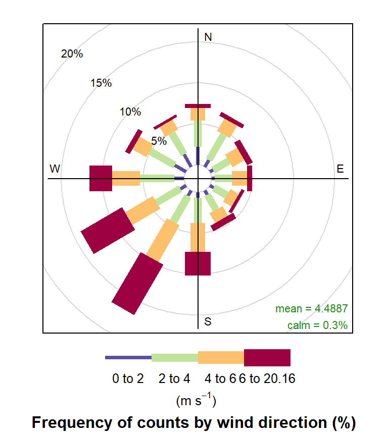
A wind rose summarising the wind conditions at a monitoring station.
However, the real flexibility comes from being able to use the type option.
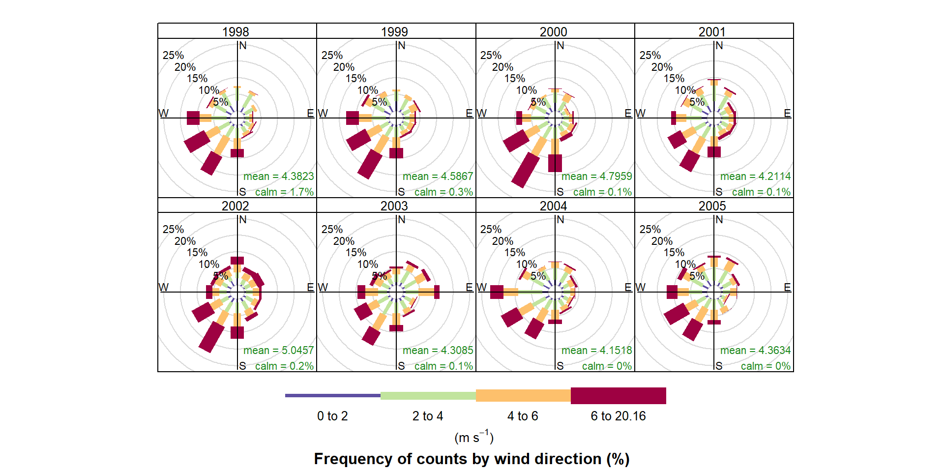
Wind roses summarising the wind conditions at a monitoring station per year, demonstrating the openair type option.
There are many flavours of bivariate polar plots, as described here that are useful for understanding air pollution sources.
polarPlot(mydata,
  pollutant = "so2",
  statistic = "cpf",
  percentile = 90,
  cols = "YlGnBu"
)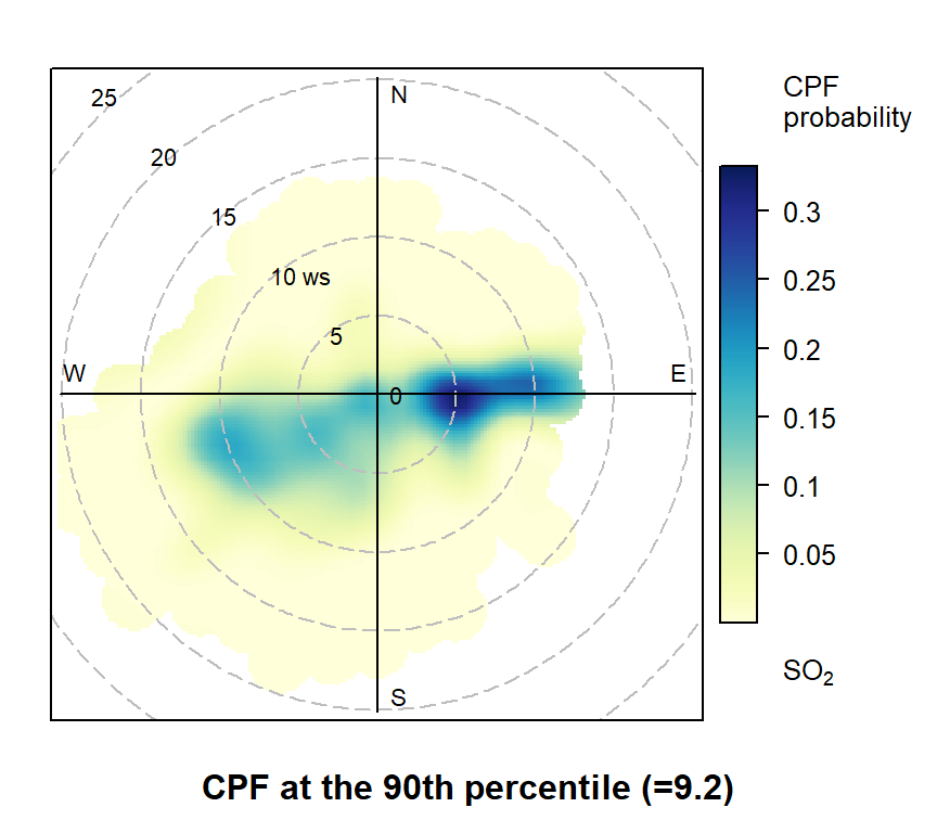
A bivariate polar plot showing the wind conditions which give rise to elevated pollutant concentrations.