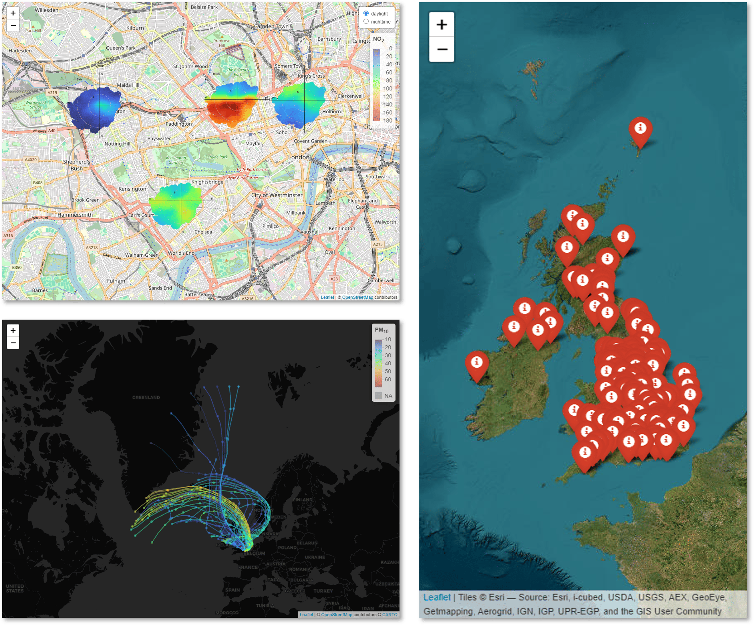
The main goal of openairmaps is to combine the robust analytical methods found in {openair} on a range of dynamic and static maps. Core functionality includes visualising UK AQ networks (networkMap()), putting “polar directional markers” on maps (e.g., polarMap()) and overlaying HYSPLIT trajectories on maps (e.g., trajMap()), all using the leaflet package. Static equivalents of most functions are also available for insertion into traditional reports and academic articles.
Installation
You can install the release version of openairmaps from CRAN with:
install.packages("openairmaps")You can install the development version of openairmaps from GitHub with:
# install.packages("pak")
pak::pak("davidcarslaw/openairmaps")
Documentation
All functions in openairmaps are thoroughly documented. The openairmaps website contains all documentation and a change log of new features. There are also many examples of openairmaps functionality the openair book, which goes into great detail about its various functions.
The {openair} toolkit
{openair}: Import, analyse, and visualise air quality and atmospheric composition data.{worldmet}: Access world meteorological data from NOAA’s Integrated Surface Database.{openairmaps}: Visualise air quality data on interactive and static maps.{deweather}: Use machine learning to remove the effects of meteorology on air quality time series.