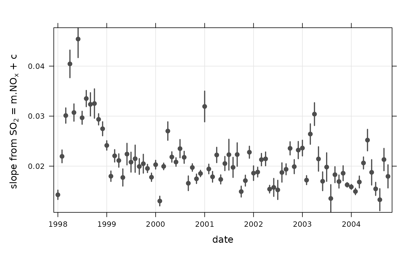
Linear relations between pollutants

This function considers linear relationships between two pollutants. The relationships are calculated on different times bases using a linear model. The slope and 95% confidence interval in slope relationships by time unit are plotted in many ways. The function is particularly useful when considering whether relationships are consistent with emissions inventories.

Usage

linearRelation(
  mydata,
  x = "nox",
  y = "no2",
  period = "month",
  condition = FALSE,
  n = 20,
  rsq.thresh = 0,
  ylab = paste0("slope from ", y, " = m.", x, " + c"),
  auto.text = TRUE,
  cols = "grey30",
  date.breaks = 5,
  plot = TRUE,
  ...
)

Arguments

mydata: A data frame minimally containing date and two pollutants.
x: First pollutant that when plotted would appear on the x-axis of a relationship e.g. x = "nox".
y: Second pollutant that when plotted would appear on the y-axis of a relationship e.g. y = "pm10".
period: A range of different time periods can be analysed. The default is month but can be year and week. For increased flexibility an integer can be used e.g. for 3-month values period = "3 month". Other cases include "hour" will show the diurnal relationship between x and y and “weekday” the day of the week relationship between x and y. “day.hour” will plot the relationship by weekday and hour of the day.
condition: For period = "hour", period = "day" and period = "day.hour", setting condition = TRUE will plot the relationships split by year. This is useful for seeing how the relationships may be changing over time.
n: The minimum number of points to be sent to the linear model. Because there may only be a few points e.g. hours where two pollutants are available over one week, n can be set to ensure that at least n points are sent to the linear model. If a period has hours < n that period will be ignored.
rsq.thresh: The minimum correlation coefficient (R2) allowed. If the relationship between x and y is not very good for a particular period, setting rsq.thresh can help to remove those periods where the relationship is not strong. Any R2 values below rsq.thresh will not be plotted.
ylab: y-axis title, specified by the user.
auto.text: Either TRUE (default) or FALSE. If TRUE titles and axis labels will automatically try and format pollutant names and units properly e.g. by subscripting the ‘2’ in NO2.
cols: Colour for the points and uncertainty intervals.
date.breaks: Number of major x-axis intervals to use. The function will try and choose a sensible number of dates/times as well as formatting the date/time appropriately to the range being considered. This does not always work as desired automatically. The user can therefore increase or decrease the number of intervals by adjusting the value of date.breaks up or down.
plot: Should a plot be produced? FALSE can be useful when analysing data to extract plot components and plotting them in other ways.
...: Other graphical parameters. A useful one to remove the strip with the date range on at the top of the plot is to set strip = FALSE.

Value

an openair object

Details

The relationships between pollutants can yield some very useful information about source emissions and how they change. A scatterPlot between two pollutants is the usual way to investigate the relationship. A linear regression is useful to test the strength of the relationship. However, considerably more information can be gleaned by considering different time periods, such as how the relationship between two pollutants vary over time, by day of the week, diurnally and so on. The linearRelation function does just that - it fits a linear relationship between two pollutants over a wide range of time periods determined by period.

linearRelation function is particularly useful if background concentrations are first removed from roadside concentrations, as the increment will relate more directly with changes in emissions. In this respect, using linearRelation can provide valuable information on how emissions may have changed over time, by hour of the day etc. Using the function in this way will require users to do some basic manipulation with their data first.

If a data frame is supplied that contains nox, no2 and o3, the y can be chosen as y = "ox". In function will therefore consider total oxidant slope (sum of NO2 + O3), which can provide valuable information on likely vehicle primary NO emissions. Note, however, that most roadside sites do not have ozone measurements and calcFno2 is the alternative.

Author

David Carslaw

Examples

# monthly relationship between NOx and SO2 - note rapid fall in
# ratio at the beginning of the series
linearRelation(mydata, x = "nox", y = "so2")

# monthly relationship between NOx and SO2 - note rapid fall in
# ratio at the beginning of the series
if (FALSE) linearRelation(mydata, x = "nox", y = "ox") # \dontrun{}

# diurnal oxidant slope by year # clear change in magnitude
# starting 2003, but the diurnal profile has also changed: the
# morning and evening peak hours are more important, presumably
# due to change in certain vehicle types
if (FALSE) linearRelation(mydata, x = "nox", y = "ox", period = "hour", condition = TRUE) # \dontrun{}

# PM2.5/PM10 ratio, but only plot where monthly R2 >= 0.8
if (FALSE) linearRelation(mydata, x = "pm10", y = "pm25", rsq.thresh = 0.8) # \dontrun{}